
Reserve markets#
License |
yes |
Release version |
10.6.1 |
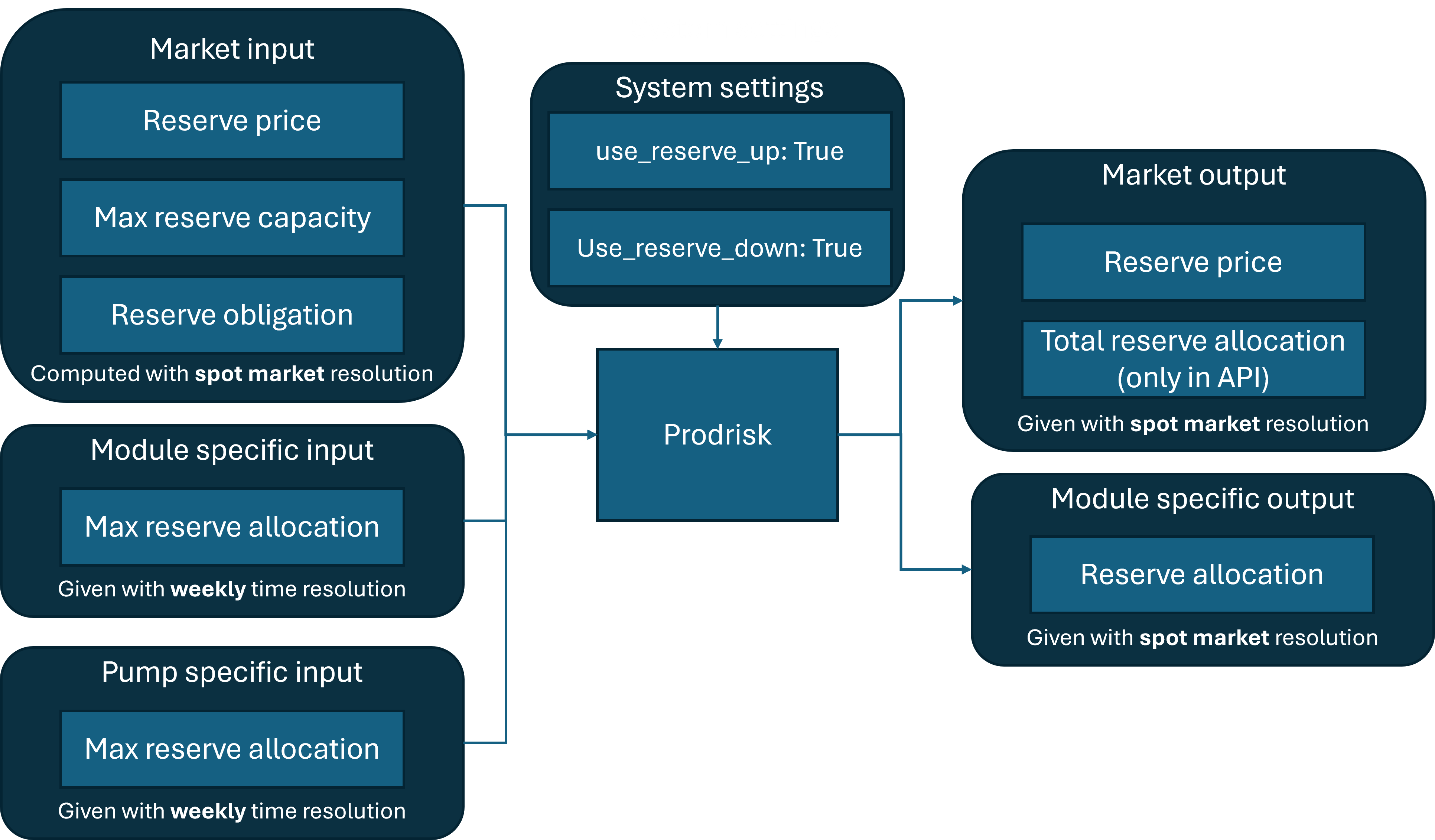
The multi-market functionality enables Prodrisk to account for reserve sales in the optimization and cut calculation. Two reserve markets are implemented, one for up regulation and one for down regulation. For each reserve market, one can specify the maximum market capacity, an obligation to be fulfilled, the reserve price, the maximum allocation per module and pump, and penalty values. All of these are time-dependent. Market input can be given with custom resolution, but will be automatically converted to the same price periods as defined for the spot market.
Outputs are the reserve allocations per module per price period. Pump results are stored in the module that the pump belongs to. Prodrisk also returns the reserve price as used in the optimization, i.e., with spot price resolution.
This is a licensed functionality that is made available on purchase.
Assumptions#
The reserve price is deterministic (same in each scenario).
Sales on all markets happen at the same time with spot price resolution.
There is no activation of reserves.
Theory#
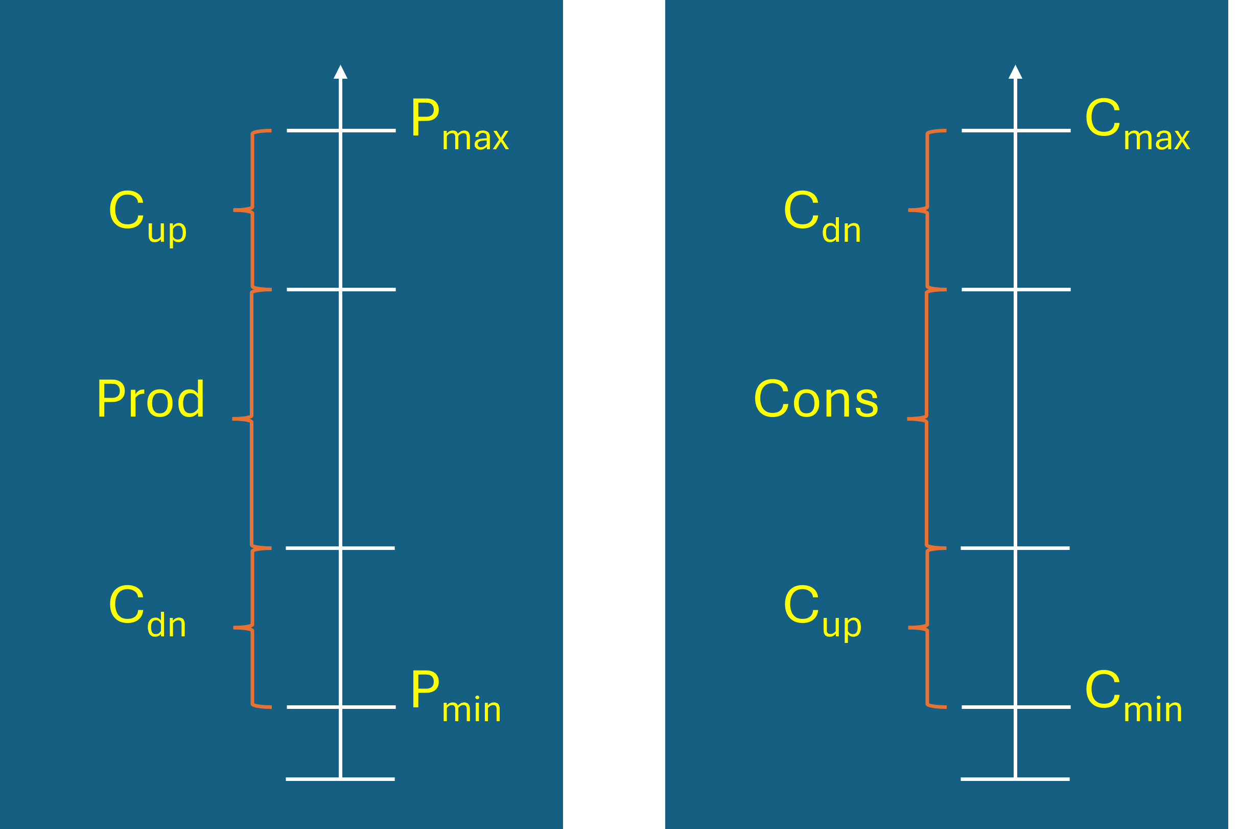
Up and down regulation capacity can be allocated by modules and by pumps in Prodrisk, as illustrated below.
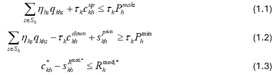
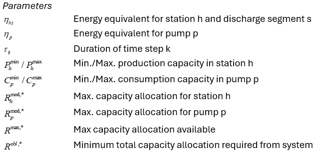
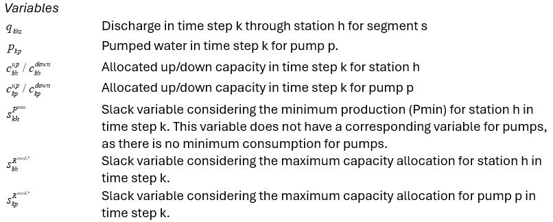
The inclusion of capacity allocation for up and down regulation markets in Prodrisk consists of adding a set of new constraints and corresponding variables to the model. Equations 1.1 and 1.2 are the maximum and minimum production constraints, respectively, of each hydropower station. The unit of these equations are GWh. 1.3 is the maximum allocation constraint, given per hydropower station, with unit MW.
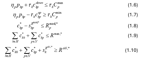
1.6 and 1.7 describe the up and down regulation capacities, in GWh, of the system pumps. 1.8 describe the maximum allocation constraint, given per pump, in MW. 1.9 and 1.10 are the market capacity constraint and obligation constraint, respectively, with unit MW.
Input format#
To activate the use of reserve markets, set use_reserve_up and/or use_reserve_down to 1 in the API, or in the file prodrisk.cpar when running from the command line. In the API, reserve market inputs are given as time-series attributes on the area object: reserve_up_price, total_reserve_up_capacity, reserve_up_obligation, reserve_up_obligation_cost, and analogously for reserve_down_*.
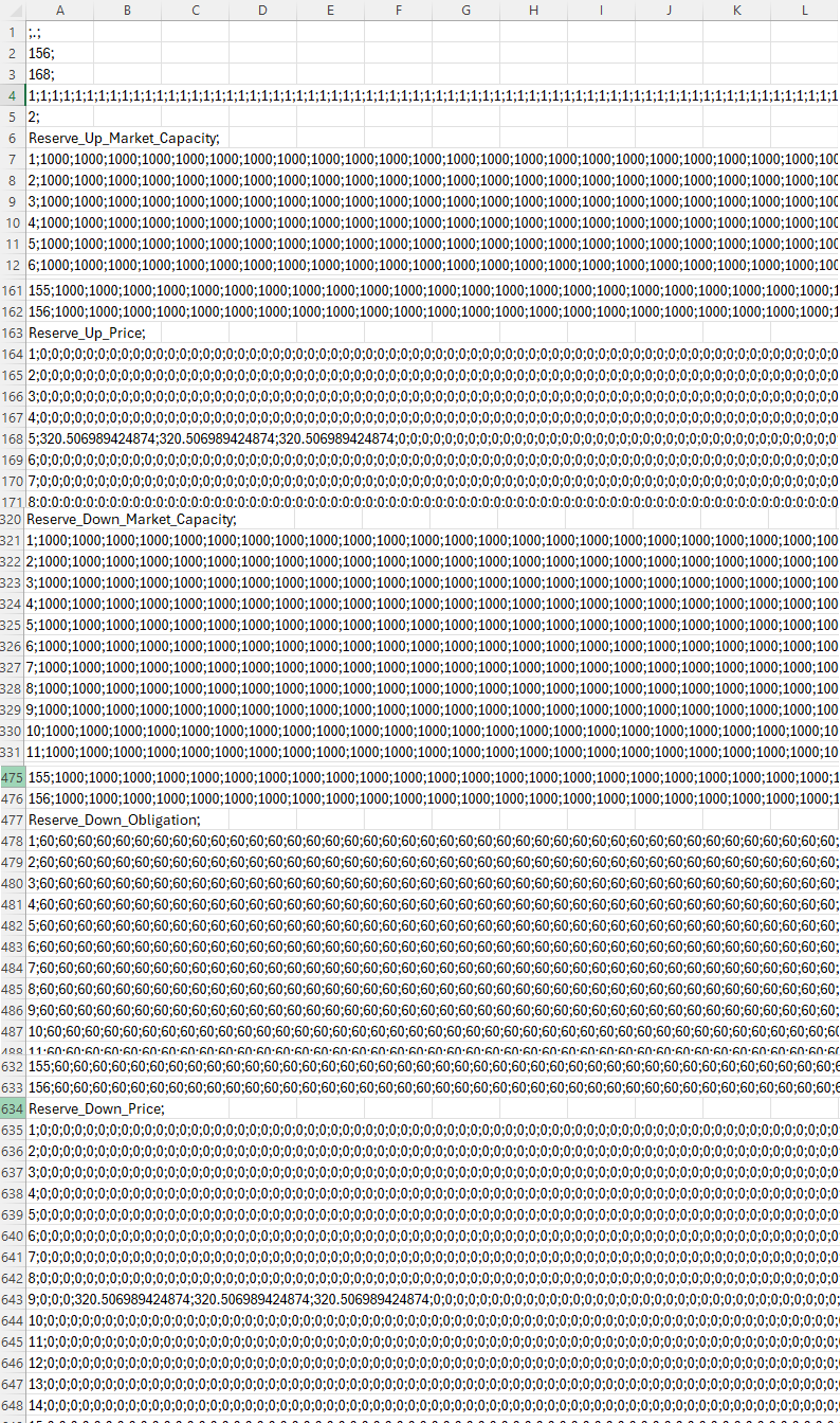
When running from the command line, these inputs are contained in the new input file Reserve.csv, with corresponding attributes: Reserve_Up_Price, Reserve_Up_Market_Capacity, Reserve_Up_Obligation, Reserve_Up_Obligation_Penalty, and analogously for Reserve_Down_*. The file format is shown below:
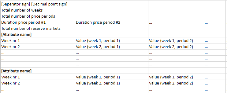
If only one value is given for a week, the same value is used for all price periods. If a week is omitted, the previous week is repeated. Default values are constant zero for obligation and price, and 30% of CTANK for the obligation cost. The market capacity is mandatory input.
The inputs on the module level have weekly resolution, and are given through new input attributes max_reserve_up, max_reserve_up_cost, max_reserve_down, max_reserve_down_cost in the API. Default values are zero for the allocation limits, and 50% of CTANK for the associated costs.
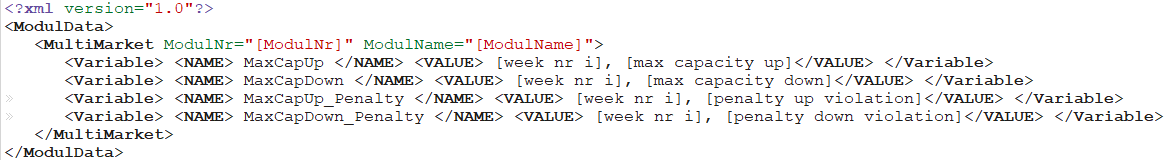
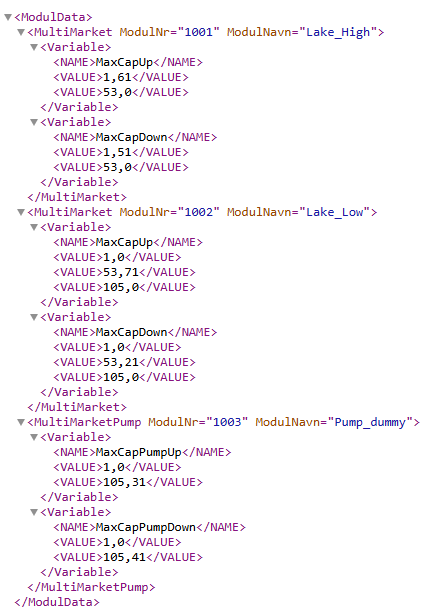
When running from the command line, the new inputs are given in constraints.xml, with corresponding attributes: MaxCapUp, MaxCapPumpUp, MaxCapUp_Penalty, MaxCapDown, MaxCapPumpDown and MaxCapDown_Penalty. The file format is shown below:
Output format#
The allocation per module per price period for each reserve market is accessed in the API through the attributes reserve_up_allocation and reserve_down_allocation, or in detsimres.h5 under hydro_module_results as up_regulation and down_regulation The pump results are stored with the module that the pump belongs to. Therefore, separate pump values are found when a pump dummy module is used. In the API there are additional area attributes total_reserve_up_allocation, total_reserve_down_allocation for the summed allocation of the whole system. The reserve prices with spot price resolution are written to the output attributes output_reserve_up_price, output_reserve_down_price on the area object, and to ENMRES.h5.
Calculation time#
The impact of calculation time mainly depends on (1) the number of modules participating in the reserve market and (2) the relation of market limits and module limits. In a system where the majority of plants can sell reserves, a loose market limit (larger than the summed allocatable capacity of all module) may lead to an increase of calculation time on the order of 20%. In contrast, a tight market limit (similar to or below the summed allocatable capacity) can increase calculation times drastically (doubling is possible). Note that the optimization is more complex in the latter case: The solver finds the optimal distribution of the market limit on the available modules. Thus, users who already know this distribution from experience can save calculation time by setting module limits that sum up to the intended market limit, while setting a loose bound on the market. The calculation time has not been tested for the inclusion of pumps in multi market allocation.
Example#
In this example, we show how to prepare input for a simple Prodrisk run with reserve markets, both through input files and in pyprodrisk. We consider a system with both up and down regulation, and the following dummy data:
Modules: Lake_High with id 1001, Lake_Low with id 1002 and Pump_dummy with id 1003
Pump: RPK_pump pumping water fram Lake_Low to Lake_High with production belonging to Pump_dumy.
Price periods: \(56\) sequential periods with lengths \(3\)
Number of weeks: \(156\)
Market capacity:
Up regulation: \(1000\) (constant)
Down regulation: \(1000\) (constant)
Market obligation:
Up regulation: \(0\) (constant)
Down regulation: \(60\) (constant)
Reserve price:
0 except for one spike for up regulation and one for down regulation, set to \(320.51\) (the maximum value of the spot price series, plus \(50\))
Week 5:
Up regulation: \(320.51\) for the first three hours
Weeks 9:
Down regulation: \(320.51\) for hours 4-6
Lake_High: Maximum allocation:
Up regulation: \(61\) (weeks 1-52), \(0\) (weeks 53-156)
Down regulation: \(51\) (weeks 1-52), \(0\) (weeks 53-156)
Lake_Low: Maximum allocation:
Up regulation: \(0\) (weeks 1-52), \(71\) (weeks 53-104), \(0\) (weeks 105-156)
Down regulation: \(0\) (weeks 1-52), \(21\) (weeks 53-104), \(0\) (weeks 105-156)
RPK_pump: Maximum allocation:
Up regulation: \(0\) (weeks 1-104), \(31\) (weeks 105-156)
Down regulation: \(0\) (weeks 1-104), \(41\) (weeks 105-156)
When running Prodrisk from the command line, we need to edit prodrisk.CPAR and constraints.xml, as well as creating the new file Reserve.csv.
prodrisk.CPAR#
In prodrisk.CPAR, we activate up and down regulation by setting
use_reserve_up 1,
use_reserve_down 1,
constraints.xml#
In constraints.xml, the module-specific reserve market input is written:
Reserve.csv#
The remaining input is written in the new file Reserve.csv (cut for illustration):
PyProdrisk#
When using pyprodrisk, we activate up and down regulation through the setting attributes use_reserve_up and use_reserve_down. Reserve market input is written to a series of txy attributes:
prodrisk.use_reserve_up = 1
prodrisk.use_reserve_down = 1

##  Example with time varying reserve up capacity
# area.total_reserve_up_capacity.set(pd.Series(name=0.0,
#                          index = [prodrisk.start_time + pd.Timedelta(weeks=i) for i in [0, 6]],
#                          data=[100.0, 120.0]))
area.total_reserve_up_capacity.set(pd.Series(name=0.0,
                         index = [prodrisk_session.start_time + pd.Timedelta(weeks=i) for i in [0]],
                         data=[1000.0]))

area.reserve_down_obligation.set(pd.Series(name=0.0,
                         index = [prodrisk_session.start_time + pd.Timedelta(weeks=i) for i in [0]],
                         data=[60.0]))

price_top = area.price.get().max().max()


## Examples with varying price
# area.reserve_up_price.set(pd.Series(name=0.0,
#                         index = [prodrisk.start_time + pd.Timedelta(weeks=i) for i in [0, 6]],
#                         data=[100.0, 120.0]))
#
# area.reserve_up_price.set(pd.Series(name=0.0,
#                         index = [prodrisk.start_time + pd.Timedelta(weeks=w) + pd.Timedelta(hours=i) for w in range(10) for i in [0,42,84,126,150]],
#                         data=[12.0, 12.0, 12.0, 8.0,  8.0,
#                               12.0, 12.0, 12.0, 8.0,  8.0,
#                               12.0, 12.0, 12.0, 8.0,  8.0,
#                               12.0, 12.0, 12.0, 8.0,  8.0,
#                               12.0, 12.0, 12.0, 8.0,  8.0,
#                               12.0, 12.0, 12.0, 8.0,  8.0,
#                               12.0, 12.0, 12.0, 8.0,  8.0,
#                               12.0, 12.0, 12.0, 8.0,  8.0,
#                               15.0, 15.0, 15.0, 10.0, 10.0,
#                               15.0, 15.0, 15.0, 10.0, 10.0]))

area.total_reserve_down_capacity.set(pd.Series(name=0.0,
                         index = [prodrisk.start_time + pd.Timedelta(weeks=i) for i in [0]],
                         data=[1000.0]))

## Example with varying price
# area.reserve_down_price.set(pd.Series(name=0.0,
#                         index = [prodrisk.start_time + pd.Timedelta(weeks=w) + pd.Timedelta(hours=i) for w in range(10) for i in [0,42,84,126,150]],
#                         data=[12.0, 12.0, 12.0, 8.0,  8.0,
#                               12.0, 12.0, 12.0, 8.0,  8.0,
#                               12.0, 12.0, 12.0, 8.0,  8.0,
#                               12.0, 12.0, 12.0, 8.0,  8.0,
#                               12.0, 12.0, 12.0, 8.0,  8.0,
#                               12.0, 12.0, 12.0, 8.0,  8.0,
#                               12.0, 12.0, 12.0, 8.0,  8.0,
#                               12.0, 12.0, 12.0, 8.0,  8.0,
#                               15.0, 15.0, 15.0, 10.0, 10.0,
#                               15.0, 15.0, 15.0, 10.0, 10.0]))

#Lake High
modA = prodrisk_session.model.module["Lake_High"]
modA.max_reserve_up.set(pd.Series(name=0.0,
                        index = [prodrisk_session.start_time + pd.Timedelta(weeks=i) for i in [0, 52]],
                        data=[61.0, 0.0]))
modA.max_reserve_down.set(pd.Series(name=0.0,
                        index = [prodrisk_session.start_time + pd.Timedelta(weeks=i) for i in [0, 52]],
                        data=[51.0, 0.0]))

#Lake Low
modB = prodrisk_session.model.module["Lake_Low"]
modB.max_reserve_up.set(pd.Series(name=0.0,
                        index = [prodrisk_session.start_time + pd.Timedelta(weeks=i) for i in [0, 52, 104]],
                        data=[0.0, 71.0, 0.0]))
modB.max_reserve_down.set(pd.Series(name=0.0,
                        index = [prodrisk_session.start_time + pd.Timedelta(weeks=i) for i in [0, 52, 104]],
                        data=[0.0, 21.0, 0.0]))

#Pump
pump = prodrisk_session.model.pump["RPK_pump"]
pump.max_reserve_up.set(pd.Series(name=0.0,
                        index = [prodrisk_session.start_time + pd.Timedelta(weeks=i) for i in [0, 104]],
                        data=[0.0, 31.0]))
pump.max_reserve_down.set(pd.Series(name=0.0,
                        index = [prodrisk_session.start_time + pd.Timedelta(weeks=i) for i in [0, 104]],
                        data=[0.0, 41.0]))