Inflow models used in Prodrisk#
The theory behind the autoregressive inflow model and the 3-parameter lognormal distribution is described more thorougly in the openly available HydroCen report [4]. More reading about the principal component analysis and residual inflow model can be done in [2].
In Prodrisk, we use time series of historically observed, predicted or estimated inflow in the forward simulations. In the backward recursion, we need a discrete mathematical model that can provide us with inflow estimates derived from the time series used in the forward simulation. The inflow model used in the Prodrisk backward iterations is a model there the inflow in one week depends on the inflow in the previous weeks, with a choice of different noise alternatives that come with different properties.
Prodrisk assumes that the inflow input is non-negative.
Autoregressive inflow model#
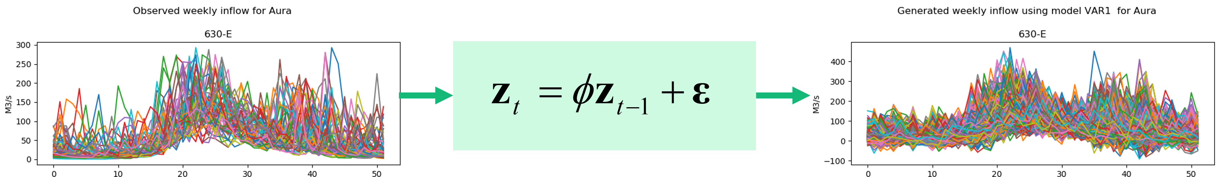
As Prodrisk is based on the SDDP algorithm, it demands a convex inflow model. To reduce complexity, the de facto inflow model is a variant of the autoregressive model. In ProdRisk, the choice is a first order vector autoregressive (VAR1) model. It means that the inflow in week t depends on the inflow from week t-1 from all available inflow series.
Assuming that only one inflow season is used, all inflow observations i from all weeks t and all series (omitting the serial index n) are standardized using the mean and standard deviation for the respective week and inflow series:
A parameter matrix \(\phi\) for a VAR1 model is then fitted to the standardized observations. The diagonal values of the parameter matrix are the autocorrelations - the contribution to this week’s inflow series i by last week’s inflow series i - and the values on the upper and lowe triangles are the cross correlations - the contributions to this week’s inflow series i by last week’s inflow from all other inflow series, respectively. If the inflow series are divided into seasons, one parameter matrix will be fitted per season.
The noice element of the VAR1 model is supposed to be a standard normally distributed variable \(\varepsilon \sim N(0,1)\) and in ProdRisk, we estimate it using three different methods:
fitting the residuals to a lognormal distribution
using principal component analysis based on the residuals
sampling directly from residuals
Lognormal inflow model (default)#
License |
yes |
Release version |
10.8 |
In the lognormal inflow model, the residuals are fitted to a 3-parameter lognormal distribution where the three parameters demand that:
the mean value of the noise model distribution should equal the mean value of the residual samples
the standard deviation of the noise model distribution should equal the standard deviation of the residual samples
the inflow generated with 3-parameter lognormal noise should be nonnegative
This results in the following definition of the noise \(\varepsilon\):
Where \(\delta\), \(\sigma\) and \(\mu\) are defined based on the observed inflow series and \(\xi \sim N(0,1)\), spatially correlated between the inflow series.
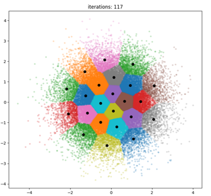
Sampling with the K-means clustering algorithm#
As one element of the three parameter lognormal noise distribution is a standard normally distributed random variable, a discrete inflow model must include sampling of some sort. Simple random sampling, which means just sampling N times and using these values directly, will only represent the distribution when \(N \rightarrow \inf\). However, a too high number of noise samples would make the calculation time of the Prodrisk backward iterations unbearably high. To generate a scenario tree using a VAR1 inflow model with 3-parameter lognormal noise distribution, a small set of inflow noise samples must represent a larger probability range. A large number of normal spatial uncorrelated noise samples can be reduced using a clustering method, for instance the K-means clustering method. The clustering method means that the large, equiprobable set of residuals is reduced to smaller, non-equiprobable set. The uncorrelated clustered sample is then transformed to spatially correlated noise using the spatial correlation of the observed residuals.
The user defines the number of samples (N_KMEANS) and the number of clusters (number of noise alternatives) in the input to Prodrisk.
Using the lognormal inflow model#
The lognormal inflow model is planned to be the default choice of inflow models as it:
Presents an expectation right inflow model
Does not produce negative inflow samples
In the API, the lognormal inflow model is chosen by setting the attribute inflow_model to “lognormal”. When running Prodrisk from the command line, the control parameter LOGNORMAL_INFLOW is set to 1 in prodrisk.CPAR.
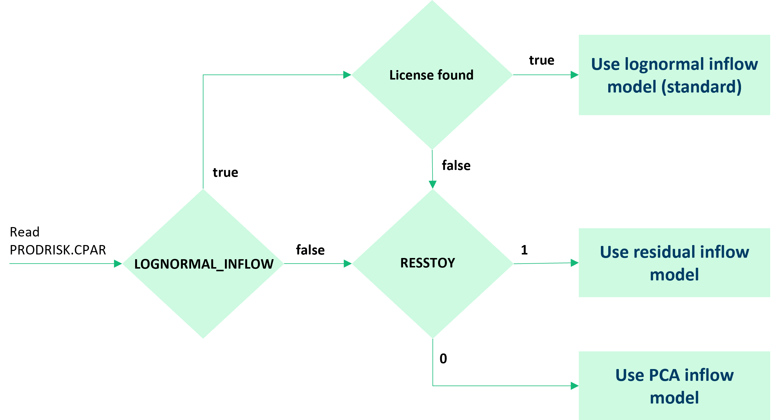
As the lognormal inflow model is the default version, the use of no prodrisk.CPAR-control parameters will result in the use of the lognormal inflow model. However, as this functionality is licensed, the absence of a license will make the value of LOGNORMAL_INFLOW irrelevant and the value of RESSTOY will decide the choice of inflow model, see Inflow model flow chart. The number of noise alternatives is set in tilsigsddp.CPAR.
Re-using the lognormal inflow model from a previous run#
Due to possibly high calculation times for the k-means clustering algorithm, it is possible to re-use the lognormal inflow model from a previous Prodrisk run. This also removes possible differences in the results between runs, appearing from the randomness in the k-means clustering.
In the API, center points and corresponding probabilities from the k-means clustering algorithm can be read from the attributes lognormal_centers, on the inflowSeries object, and lognormal_probabilities, on the area object. The same attributes must be set when re-using the inflow model in a later Prodrisk run, as well as the attribute read_lognormal_model which must be set to 1.
When running Prodrisk from the command line, Prodrisk writes the file lognormalInflowModel.h5 containing center points and corresponding probabilities from the k-means clustering. In order to re-use the inflow model in a later Prodrisk run, the parameter READ_INFLOW_H5 is set to 1 in prodrisk.CPAR. Prodrisk will then read from lognormalInflowModel.h5 instead of repeating the clustering procedure. If the file does not exist and READ_INFLOW_H5 is set to 1, an error message will be written to the log file, and Prodrisk will generate a new inflow model.
Principal component analysis#
The principal component analysis identifies the NPRBRUK components contributing most to the total variance of the samples, transform the sample space into a reduced set of dimensions and transform back again a discrete set of points representing the distribution of each principal component of the samples. After the principal component analysis, a small set of discrete points representing the whole sample distribution is used as noise for the autoregressive inflow model.
Using the principal component analysis inflow model#
The principal component analysis inflow model is the temporary default inflow model and the second option, carrying the properties that it:
Presents an expectation right inflow model
Can produce negative inflow samples
In the API, the principal component analysis inflow model is chosen by setting the attribute inflow_model to “principal”. When running Prodrisk from the command line, the control parameter LOGNORMAL_INFLOW is set to 0, and RESSTOY is undefined or set to 0 in prodrisk.CPAR. The number of principal componets used and the number of discrete values per principal component are set in tilsigsddp.CPAR.
Residual model#
An alternative way to obtain the noise \(\varepsilon\) is to sample directly from the residuals using simple random sampling. With a high enough number of noise samples, this method would represent the whole distribution of the residuals from the inflow series. However, with a small number of noise samples, the simple random sampling will not produce expectation right inflow. On the other hand, the inflow generated with the residual model can be tested for negativity, and these generated inflow samples can be corrected.
Using the residual inflow model#
The residual inflow model is the third available option:
Does not produce expectation right inflow
Can be corrected for negative inflow
In the API, the residual inflow model is chosen by setting the attribute inflow_model to “residual”. When running Prodrisk from the command line, the control parameter LOGNORMAL_INFLOW is set to 0, and RESSTOY is set to 1 in prodrisk.CPAR. The number of noise alternatives is set in tilsigsddp.CPAR.
Inflow model flow chart#
The default inflow model is the lognormal inflow model, which requires a licence.