Prodrisk penalty information#
A constraint may be violated with the corresponding added cost in the objective function if the gain is higher than the penalty cost involved. Therefore, it is imperative to calibrate the penalties carefully. However, calibration of the different penalties is non-trivial, especially for complicated watercourse topologies. To aid the user in this process, improved information is presented to help the user understand how a choice of penalty parameters affect the solution of the optimization.
These new files are generated:
constraints.txt
constraintViolation.txt
InflowStatistics.txt
penalty.txt
Previously, accumulated constraint violations from the final simulation have been shown in command line window when Prodrisk has been run. In the print-out, this information is accompanied by detailed information about constraint violations distributed on modules, simulation scenarios and simulation weeks from the final simulation, along with detailed information about constraint violations from the backward iterations as well.
The system constraints and penalty values are constant throughout the program and are printed after the Prodrisk iterations are done. The constraint violations are logged internally as the program progresses, but are also printed out in the end.
How do I use this feature?#
Set write_penalty_logfiles to 1 (in the file PRODRISK.CPAR, or set the attribute in the API). The visualisation of penalties in Prodrisk does not affect the optimization, but since the information must be added in the parallel processing communication it may increase the computation time slightly. By default this feature is therefore turned off. Constraint violations are logged during the final simulation or the backward iterations, but writing to file happens when the iterations are done. The new text files will be created in your run folder. A subset of the information on these files are available as result attributes in the API.
Constraints#
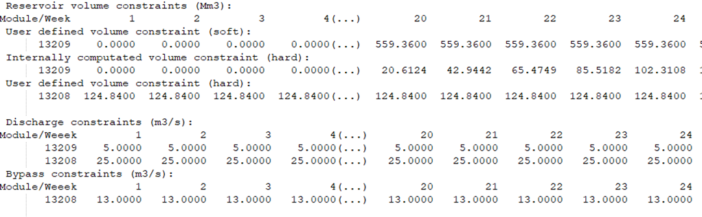
The text file constraints.txt shows the minimum reservoir constraints, the minimum discharge constraints and the minimum bypass constraints for each module and for each week. The reservoir volume constraints are labelled as “User defined volume constraint (soft):”, ” Internally computed volume constraint (hard)” or “User defined volume constraint (hard)”. The intention of the soft volume constraint is that during the constraint period, the inflow to the reservoir is used to fill the reservoir and that there will not be any discharge from the reservoir, until the reservoir minimum level is reached. Once the minimum level is reached, the constraint should act like a hard constraint. In Prodrisk, this is implemented as a much lower limit that is calculated based on the mean inflow to the reservoir. This internally calculated limit acts as a hard constraint. For the discharge and bypass, there is only one type of constraint per module.
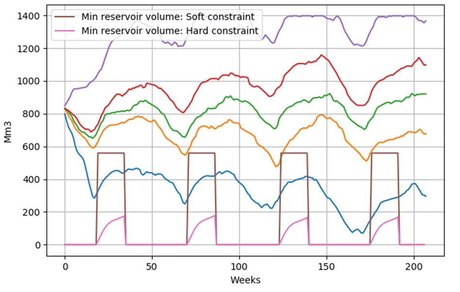
The reservoir volume constraints for module 13209 are shown in the figure below. In Prodrisk, a soft reservoir volume constraint prevents discharge from reservoir if its volume is below the soft limit (brown line). The constraint does not cause any penalties unless the volume is below the converted, hard constraint (pink line). The hard constraint is constructed based on average inflow using the following method. Assume zero storage level at the beginning of the soft constraint period and that the plant is not discharging before the required minimum reservoir level is achieved.
Constraint Violations#
The text file constraintViolation.txt contains the accumulated constraint violations from the final simulation that also appears in the printout to screen in the end of the Prodrisk session, as well as a detailed overview of the constraint violations from the final simulation listed for each week and simulation scenario.
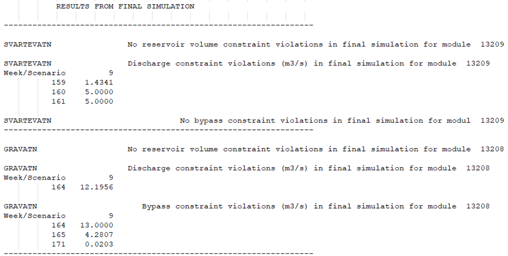
The constraint violations are organized as one matrix for each constraint type and module, listing all the constraint violations for one module before moving on to the next. For each combination of module and constraint, the occurrences of violations are shown with corresponding week, scenario and size of the constraint violation. Weeks and scenarios where no constraint violations occur are not included in the printout. The minimum reservoir constraint violations are accumulated for all price periods within the week both in the final forward simulation, for the last backward iteration and for the extra cut generation. Even though the reservoir volume by the end of the week may be within the boundary, the reservoir volume for one or more of the time periods within the week may be violated and will therefore end up in the table in constraintViolation.txt.
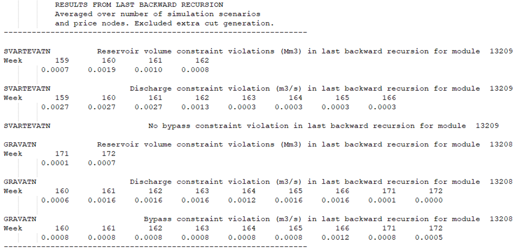
The constraint violations for the last backward recursion are not distributed on scenarios, but averaged on each week in the iteration according to the probability of each scenario. After the final backward iteration has been conducted, a set of additional cuts for extreme reservoir volumes are created in an additional backward iteration. As these cuts are prepared for the extreme situations, there is a much higher number of constraint violations.
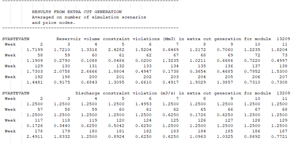
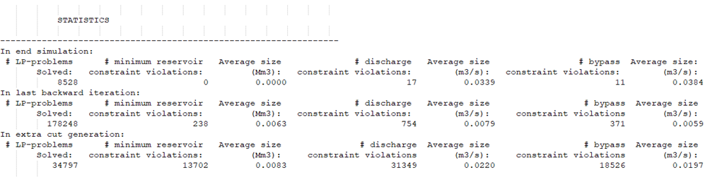
Finally, the file constraintViolation.txt shows statistics from the final simulation, the last backward recursion and the extra cut generation. These statistics include the total number of LP problems solved, the total number of constraint violations and the average size of the constraint violations of each constraint type for this iteration phase.
Penalties used in the objective function#
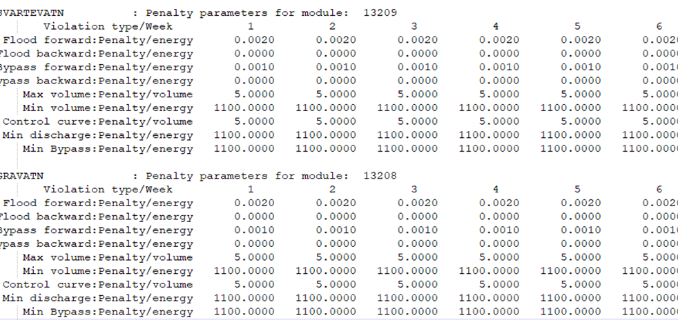
The file penalty.txt shows a print-out of the actual penalty values that are used in the Prodrisk optimization for all penalty variables, modules and simulation weeks. To set the penalty values, see the documentation on Penalty-values.
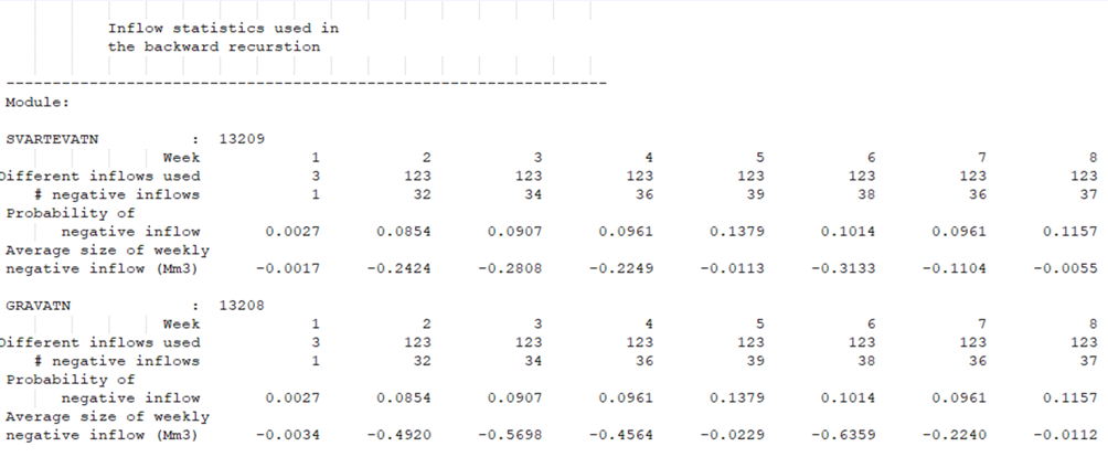
Negative inflow statistics#
The SDDP algorithm used in Prodrisk demands convexity, which motivates the use of a linear stochastic inflow model based on a first-order vector autoregressive model (VAR1) for the backward recursions. To remove seasonal variation, the observed inflow is normalized before fitting it to the VAR1 model. The autoregressive model will sometimes produce negative inflow values. It is useful to quantify the frequency and volume of the negative inflows because negative inflows may trigger use of high penalties for negative reservoir storages. As the negative inflow will be the same for all iterations, all price nodes and all trajectories, they are recorded in the first backward recursion for the first price node and trajectory but printed in the finishing simulation. A section of the file inflowStatistic.txt is shown below. For each week, the number of inflow samples used is recorded along with the number of negative inflow samples, the probability for a negative inflow and the average volume of the negative inflow for that week, whenever a negative inflow occurs. For weeks without any negative inflow samples, the probability and average volume are zero.