Inflow scaling#
In this article, we go through the units and scaling factors of input and output related to inflow to answer common questions like:
Which attributes dertermine how much water will end up in each reservoir in the simulation?
How can outputs be used to double-check the amount of water?
How do the area (global) attributes differ from the module (local) attributes?
Here we assume that pyprodrisk is used. However, the following does also apply to the corresponding command-line parameters, if Prodrisk is run with LTM_CALENDAR=TRUE on a ScenarioData.h5 file without a Forecast.h5 file. For more information on these files, inflow pre-processing and different calendar settings please consult the documentation of the LTM package, in particular the program tilpro.
Inflow input attributes and units#
We start by summarizing the input that is used to control the inflow volume in the simulation and introduce mathematical symbols used in the following sections. The meaning and use of this input is independent of the inflow model. For information on the inflow model and related settings (which we omit here), there is a separate article.
per inflow series (inflowSeries object):
seires identifier, attribute seriesId
historical average inflow \(V_\text{ser}\,\left[\mathrm{Mm^3/y}\right]\), attribute histAverageInflow
inflow scenarios \(S_i(t)\,\left[\mathrm{m^3/s}\right]\), attribute inflowScenarios
per reservoir (module object):
inflow series for regulated inflow, attribute connectedSeriesId
inflow series for unregulated inflow, attribute connected_unreg_series_id
mean annual regulated inflow volume \(V^r_\text{mod}\,\left[\mathrm{Mm^3/y}\right]\), meanRegInflow
mean annual unregulated inflow volume \(V^u_\text{mod}\,\left[\mathrm{Mm^3/y}\right]\), meanUnregInflow
The time dependence of the inflow is given through \(S_i(t)\), while the averages per series and module are used to scale the time series such that each module receives the correct amount of water. Note that usually several modules are linked to the same inflow series. If the inflow to two reservoirs only differs by a factor, it is not recommended to provide their inflow as separate – but fully correlated – series, which would give redundant information to the inflow model and also occupy more memory than needed. In such (very common) cases, the modules will use the same series, but have individual annual inflow volumes.
Regulated and unregulated inflow#
Regulated inflow is storable water that is flowing into the reservoir. It can be used to produce or bypass immediately or at a later time. Surplus inflow that exceeds the maximum reservoir capacity is spilled. Unregulated inflow, on the other hand, refers to water that cannot be stored in the reservoir. It can be used for immediate production or gets bypassed/spilled if it exceeds the maximum flow through the plant. The attributes for regulated and unregulated inflow work analogously, where connectedSeriesId and meanRegInflow refer to regulated inflow, whereas connected_unreg_series_id and meanUnregInflow refer to unregulated inflow. The series id tells Prodrisk which inflowSeries object to connect to this module. The meanRegInflow is the average annual amount of water flowing into the reservoir up to an historic scaling factor - we will return to the scaling below. Note that input for regulated inflow is mandatory. Input for unregulated inflow is optional: By default, connected_unreg_series_id is set equal to the connectedSeriesId, i.e., regulated and unregulated inflows are inferred from the same series. The meanUnregInflow is zero by default.
Historical average inflow#
The historical average inflow \(V_\text{ser}\) for each series serves as a reference value which Prodrisk relates to the annual average inflow in the inflow scenarios. The latter is calculated based on the last 52 weeks per scenario:
The factor \(f_{\Delta t}\) is needed to convert units from \(\mathrm{m^3/s}\) to \(\mathrm{Mm^3}\). Assuming that \(S_i(t)\) has daily resolution, \(f_\mathrm{day} = 3600 \cdot 24 \cdot 10^{-6} = 0{.}0864\). By default, Prodrisk will set the historical average inflow \(V_\text{ser}\) to \(\overline{S}\), but the user can set a different value, e.g., to the average from a historical period that differs from the simulation period.
Inflow scaling per module#
The average yearly inflow for a module is specified by \(V^r_\text{mod}\) and \(V^u_\text{mod}\). Importantly, these values must be based on the reference value \(V_\text{ser}\) of the connected inflow series. If the actual scenario average \(\overline{S}\) differs from \(V_\text{ser}\), then Prodrisk will scale the water received by the module accordingly relative to \(V_\text{mod}\). Let us denote the regulated inflow used in the simulation for a given module \(Z^r_i(t)\) in scenario \(i\). Then the inflow in \(\mathrm{Mm^3}\) per time step in the simulation is:
and analogous for unregulated inflow. Hence, the average yearly inflow in the simulation is:
More precisely, this is the average inflow during the last 52 weeks of the simulation period. If scenarios are constructed from consecutive weather years in the standard way, where year 2 in scenario 1 equals year 1 in scenario 2, etc., this subtlety does not matter (up to edge years). However, if the scenarios are built from independent data, like a stochastic forecast, it might be relevant that \(\overline{S}\) does not account for the whole period.
Inflow output attributes and units#
The inflow that was used in the optimization is reported back as an output by Prodrisk and can be used to check if the model was set up correctly. These outputs are stochastic time series. Keep in mind that the resolution of the output series will in general differ from the resolution of the inflow input.
for each reservoir (module object)
local inflow \(L_i(t) \, \left[\mathrm{m^3/s}\right]\), attribute localInflow. (NB: The corresponding data series in the result file detsimres.h5 is in \(\mathrm{Mm^3}\) and is converted to \(\mathrm{m^3/s}\) by the API.)
for the entire watercourse (area object)
aggregated energy inflow \(E_i(t) \, \left[\mathrm{GWh}\right]\), attribute total_storable_inflow
The attribute total_nonstorable_inflow exists but lacks implementation and should not be used.
Again, here we omit attributes related to the inflow model like information on the occurrence of negative inflow in the principal component model.
As of now, the inflow output from Prodrisk does not distinguish storable and nonstorable inflow (despite the attribute name total_storable_inflow). The output series on both area and module level are the sum of regulated and unregulated inflows.
The local inflow is by default returned with weekly resolution. If sequential resolution of module results is activated, the local inflow will have price period resolution. The API automatically returns \(L_i(t)\) in \(\mathrm{m^3/s}\), so you normally do not have to think about the factor \(f_{\Delta t}\). However, the result series in detsimres.h5 is \(Z^r_i(t) + Z^u_i(t)\) in \(\mathrm{Mm^3}\).
The aggregated energy inflow is converted to \(\mathrm{GWh}\) by multiplying the inflow with the energy equivalent \(\varepsilon \, \mathrm{GWh/Mm3}\) of the respective module, and then summed over all modules in the model. For simplicity, we suppress extra module indices.
\(E_i(t)\) has always price period resolution.
Example 1: One module with regulated and unregulated inflow#
Let us assume that we have a Prodrisk session called prodrisk with a module called Module-A and two inflow series, Serie-1 and Serie-2. We do not set histAverageInflow for the series, so it will be set automatically to \(\overline{S}\) as explained above. For the module, we set:
prodrisk.model.inflowSeries['Serie-1'].seriesId.set(1)
prodrisk.model.inflowSeries['Serie-2'].seriesId.set(2)

mod = prodrisk.model.module['Module-A']
mod.connectedSeriesId.set(1)             # Serie-1 as regulated inflow
mod.connected_unreg_series_id.set(2)     # Serie-2 as unregulated inflow
mod.meanRegInflow.set(100.0)             # 100 Mm3 regulated inflow / year
mod.meanUnregInflow.set(20.0)            #  20 Mm3 unregulated inflow / year
We do not show the rest of the input in this snippet, like reading the scenarios from some database. When the session is set up completely, we call prodrisk.run() and take a look at the output. First, how much water does actually flow to the module? We use the output localInflow and convert from \(\mathrm{m^3/s}\) to \(\mathrm{Mm^3/y}\) (one year in Prodrisk = 52 weeks).
inf = mod.localInflow.get()              # module inflow in m3/s
m3s_Mm3y = 1e-6 * 3600*168*52            # conversion factor
print(inf.mean() * m3s_Mm3y)             # annual inflow in each scenario
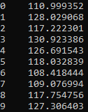
The inflow differs in each scenario (10 in this example) and is spread around the sum of regulated and unregulated inflow, \(100\,\mathrm{Mm^3} + 20\,\mathrm{Mm^3}=120\,\mathrm{Mm^3}\).
Taking the average over all scenarios, inf.mean().mean() * m3s_Mm3y, we get \(119.4\,\mathrm{Mm^3}\). This is very close to the expected average, but not exact. The reason is that we have based our average on the entire simulation period. Let us repeat the analysis restricted to the last 52 weeks, which \(\overline{S}\) is based on:
index_time = prodrisk.start_time + pd.Timedelta(weeks = prodrisk.n_weeks - 52)
print(inf[inf.index >= index_time].mean().mean() * m3s_Mm3y)
Now, the output is exactly the input value \(120\mathrm{Mm^3}\) up to numerical precision. If you still observe a deviation at this point, the reason might be that you have not set the environmental variable LTM_CALENDAR=TRUE, which is needed when using pyprodrisk.
Applying the same operation on the input series, we can also calculate \(\overline{S}\) explicitly for both series:
inf_1 = prodrisk.model.inflowSeries['Serie-1'].inflowScenarios.get()
S1 = inf_1[inf_1.index >= index_time].mean().mean() * m3s_Mm3y

inf_2 = prodrisk.model.inflowSeries['Serie-2'].inflowScenarios.get()
S2 = inf_2[inf_2.index >= index_time].mean().mean() * m3s_Mm3y
Now we expect that, in each time step, the local inflow is the sum of series 1 and 2, weighted with their scaling factors \(V^r_\text{mod}/\overline{S}_1\) and \(V^u_\text{mod}/\overline{S}_2\). Recall that, if we had set historical average inflow as input on the series, this input would be used instead of \(\overline{S}\) which is calculated internally (and usually not of interest to the user). We can make a plot to see the scaling, showing only the average over scenarios for simplicity:
scaling_1 = mod.meanRegInflow.get() / S1
scaling_2 = mod.meanUnregInflow.get() / S2

import matplotlib.pyplot as plt

# unscaled series for comparison
plt.plot(inf_1.mean(axis=1), label='Serie-1')
plt.plot(inf_2.mean(axis=1), label='Serie-2')

# scaled input
plt.plot((inf_1 * scaling_1 + inf_2 * scaling_2).mean(axis=1),label='scaled input')

# output
plt.plot(inf.mean(axis=1),':',label='local inflow') # dotted to see lines on top of each other

plt.legend()
plt.grid()
plt.show()
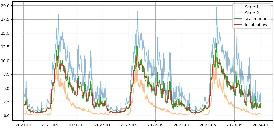
Looking at the details, one can spot that the scaled input looks a bit different from the local inflow. This is because the series have different time resolution. Without sequential resolution of module results, the local inflow has weekly resolution. Explicitly resampling everything to weekly intervals, the curves become identical:
weekly_input = (inf_1 * scaling_1 + inf_2 * scaling_2).resample('w').mean()
weekly_inf = inf.resample('w').mean()
plt.step(weekly_input.mean(axis=1),'-',label='scaled input')
plt.step(weekly_inf.mean(axis=1),':',label='local inflow')

Finally, we can check the energy inflow for the system.
area_name = prodrisk.model.area.get_object_names()[0]
area = prodrisk.model.area[area_name]
gwh_inflow = area.total_storable_inflow.get()
In this example with only one module, it is the same as the local inflow, but in \(\mathrm{GWh}\). For a simple comparison, we can again use weekly averages:
eneq = mod.energyEquivalentConst.get()
GWh_m3s = 1e6 / (7*24*3600) / eneq     # GWh/week to m3/s
area_inflow = gwh_inflow.resample('w').sum() * GWh_m3s

plt.step(area_inflow.mean(axis=1),'-',label='converted area inflow')
plt.step(weekly_inf.mean(axis=1),':',label='local inflow')

plt.legend()
plt.grid()
plt.show()
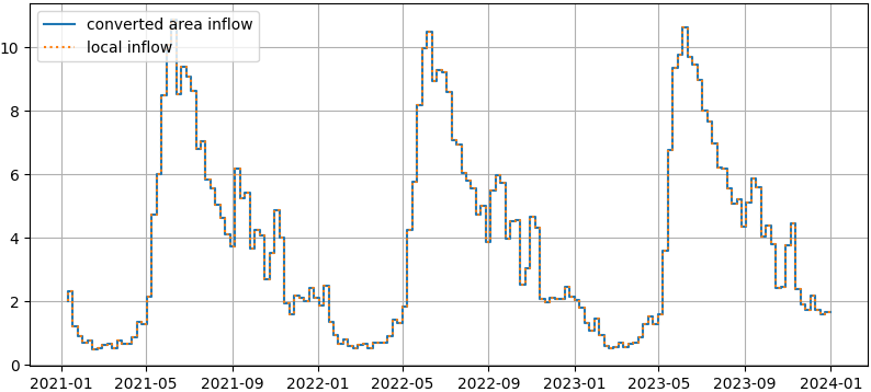
Again, the output is completely consistent. For a system with several modules, we would have to sum all local inflows to reproduce the area output.
Example 2: Historical reference values#
We use the same model as in the first example, but now with historical average values on both series. Assume that we know from historical data that if the annual average inflow in series 1 is \(250\,\mathrm{Mm^3}\), then the regulated inflow to the module is \(100\,\mathrm{Mm^3}\). If the annual average inflow in series 2 is \(80\,\mathrm{Mm^3}\), then the regulated inflow to the module is \(20\,\mathrm{Mm^3}\). Thus we set:
prodrisk.model.inflowSeries['Serie-1'].histAverageInflow.set(250)
prodrisk.model.inflowSeries['Serie-2'].histAverageInflow.set(80)

mod.meanRegInflow.set(100.0)             # as in example 1
mod.meanUnregInflow.set(20.0)            # as in example 1
Let us check how that compares to the scenario averages as calculated above:
factor_1 = S1 / prodrisk.model.inflowSeries['Serie-1'].histAverageInflow.get()
factor_2 = S2 / prodrisk.model.inflowSeries['Serie-2'].histAverageInflow.get()

print(factor_1)
print(factor_2)
The values in the inflow scenarios are clearly below the historical reference value. Therefore, we expect that the local inflow to the module is reduced by the same factors. The sum of regulated and unregulated inflow should be:
V_tot = factor_1 * mod.meanRegInflow.get() + factor_2 * mod.meanUnregInflow.get()
print(V_tot)
Repeating the steps from example 1 after the running the simulation, we can verify that this is the value used by Prodrisk:
inf = mod.localInflow.get()
print(inf[inf.index >= index_time].mean().mean() * m3s_Mm3y)